Euroleague Pythagorean Expectation
What is Pythagorean expectation? Link to heading
Pythagorean expectation is a formula that was originally derived by Bill James to be used in baseball. The objective of the formula was to estimate how many wins a team should have won based on the number of scored runs and allowed runs. You can read more about the theorem on Wikipedia and this article that also presents few practical examples. Originally the form of the formula looks like this: $$W \approx \frac{(\text{scored runs}) ^ 2}{(\text{scored runs}) ^ 2 + (\text{allowed runs}) ^ 2}\text{,}$$ where $W$ is the ratio of team’s wins or winning ratio.
However, we can generalize the above formula to other sports. If we use general notation, where $P_F$ denotes points for and $P_A$ denotes points against, then formula then converts to:
$$ W \approx \frac{{P_F} ^ x}{P_F ^ x + P_A ^ x} \text{.} $$
Notice that in the second formula the exponents are not defined. As seen in the first formula for baseball, Bill James used $x = 2$. Later there were some corrections for baseball to set $x = 1.83$. The value of $x$ depends on the nature of the sport. In football we see significantly lower number of points (goals) scored in comparison to basketball, so in order for the formula to be a good estimator of winning ratio we need to set the $x$ value correctly, which will be explained later on.
Pythagorean expectation applied to Euroleague Link to heading
In this article I will demonstrate how well Pythagorean theorem applies to basketball, specifically to the strongest european competition of Turkish Airlines Euroleague.
For the analysis I used seasons of 2016/2017, 2017/2018, 2018/2019 and 2020/2021.
Let’s draw a plot of Pythagorean expectation vs. $W$ for each team in listed seasons. Here, I used $x = 2$ just to show that we can also draw conclusions using the original $x$ value:
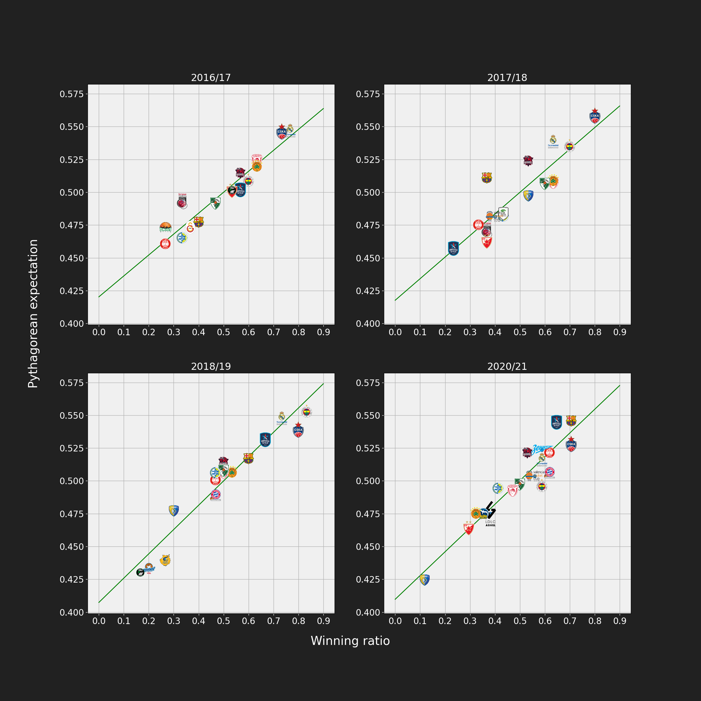
We observe that the values on vertical and horizontal axis are not in the same range, therefore we conclude that the $x = 2$ is not the best setting for this data. However, there definitely is a linear relationship between winning ratio and Pythagorean expectation. The green line in plots presents the line obtained by linear regression. Furthermore, I calculated Pearson correlation coefficients to confirm the linear relationship:
| season | corr. coef. |
|---|---|
| 2016/17 | 0.954 |
| 2017/18 | 0.887 |
| 2018/19 | 0.963 |
| 2020/21 | 0.945 |
Finding the best exponent Link to heading
We observed that there is obvious correlation between Pythagorean expectation and winning ratio, however $x = 2$ is not the choice to directly estimate $W$ from points. To get the best fit for $x$ I constructed simple loss function:
$$
L(x) = \frac{\sum_{i=1}^n | W_i - \frac{{P_{F_i}} ^ x}{P_{F_i} ^ x + P_{A_i} ^ x}|}{n} \text{.}
$$
The loss function minimizes the average difference between winning ratio and Pythagorean expectation across all teams with respect to parameter $x$. For loss function minimization I used function fmin_l_bfgs_b from scipy library. The values were calculated for each season separately:
| Season | Best x | Loss |
|---|---|---|
| 2016/17 | 11.24 | 0.034 |
| 2017/18 | 10.95 | 0.056 |
| 2018/19 | 11.03 | 0.039 |
| 2020/21 | 11.10 | 0.041 |
The best fits for each of four seasons are pretty similar, $x \approx 11$. It could be that the $L(x)$ has multiple local minima and fmin_l_bfgs_b might not have returned the global minimum. We can verify that these $x$ values are indeed the best fit with respect to $L(x)$ using brute force by simply evaluating function on range $x$ = [0, 30] with step of 0.05.
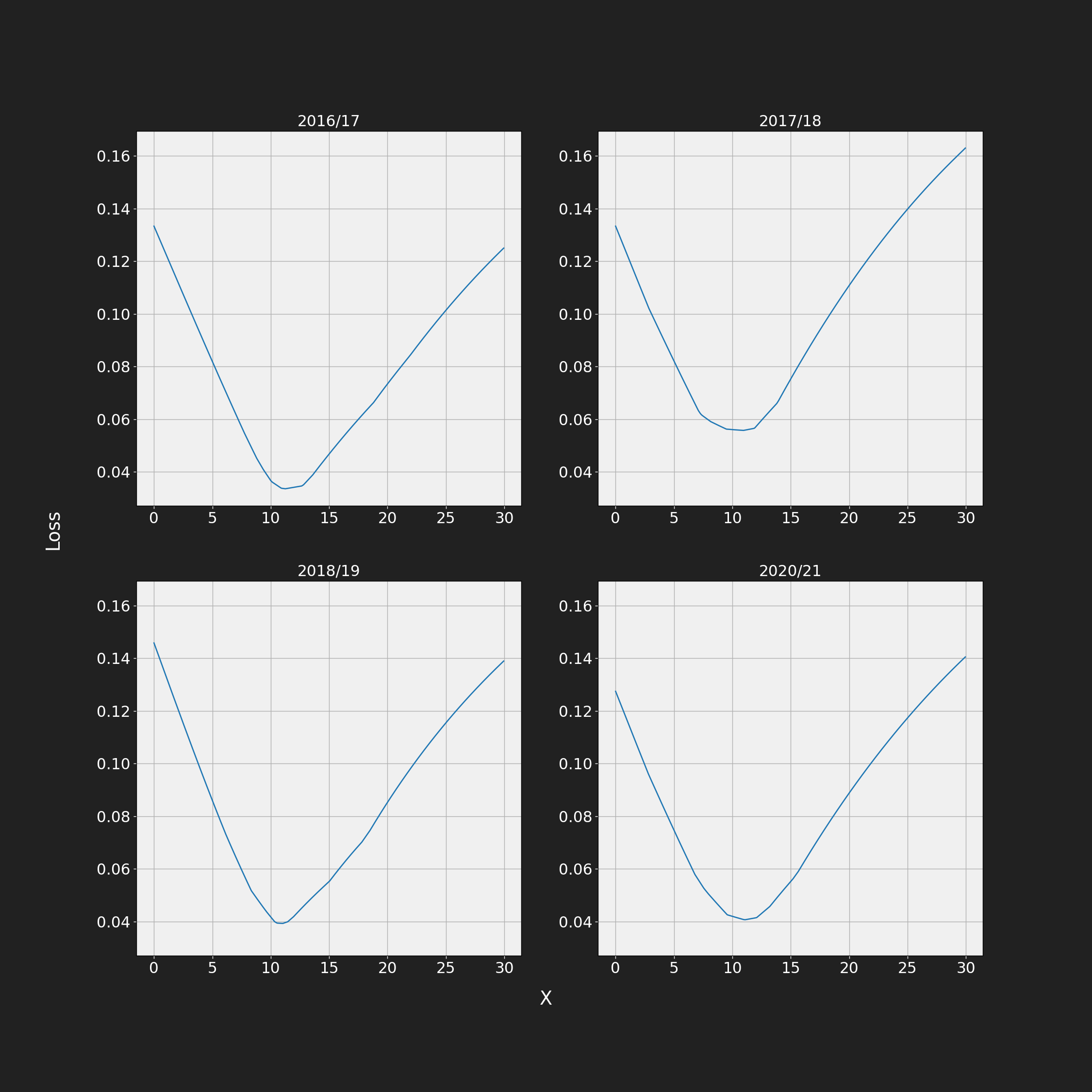
These seem to be convex functions, so there should not be any problems getting the smallest loss using any of the two methods. Quick glance at plots suffices to confirm that $x \approx 11$ seems to be a good fit for this data, however we also can also show values obtained using this method:
| Season | Best x | Loss |
|---|---|---|
| 2016/17 | 11.25 | 0.034 |
| 2017/18 | 10.95 | 0.056 |
| 2018/19 | 11.00 | 0.039 |
| 2020/21 | 11.10 | 0.041 |
Comparing both tables, we conclude that the values are more or less identical and therefore both methods are adequate for finding the best value for parameter $x$.
Utilizing the chosen $x$ Link to heading
Finally, we use the obtained $x$ values, to adjust the Pythagorean expectation in order to get the best fit for given data. Note that the green line in this case does not represent the line obtained using linear regression, it is simply just $y = x$ line.
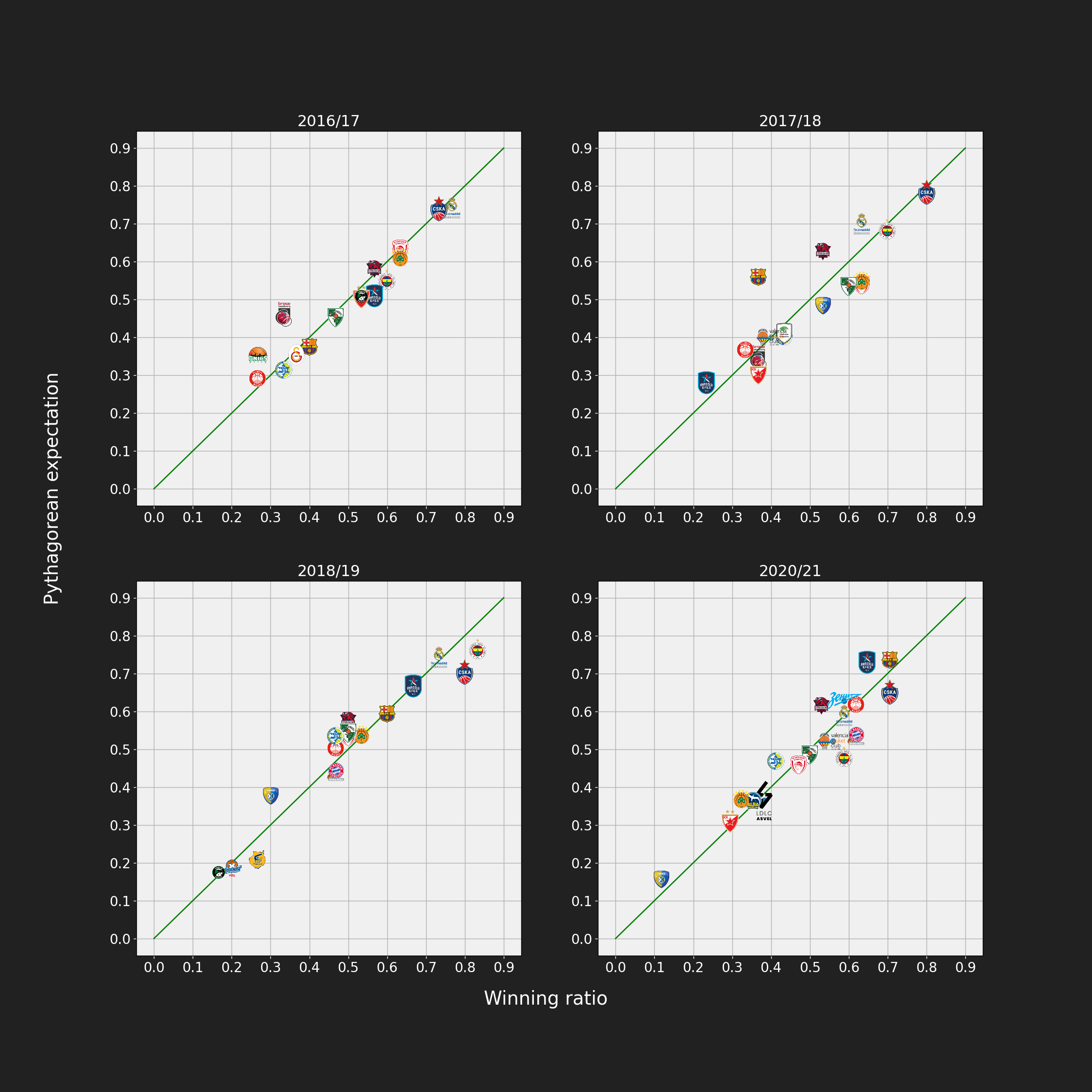
Again, we confirm strong linear correlation between Pythagorean expectation and winning ratio:
| season | corr. coef. |
|---|---|
| 2016/17 | 0.956 |
| 2017/18 | 0.884 |
| 2018/19 | 0.967 |
| 2020/21 | 0.944 |
Here, the interpretation of the plots should be the following: the teams that are above the line managed to win fewer games than expected, considering the number of scored points and allowed points. The teams that are below the line managed to win more games than expected.
Few interpretations:
- In 2017/2018 Barcelona finished 13th, however they definitely had potential to reach the Top 8.
- In 2020/2021 Fenerbahce finished 7th with winning ratio close to 0.6, but it seems that they had some luck on their side. Their expected winning ratio is below 0.5, which would leave them without Top 8.
You can find all the code for this article in my Github repository.